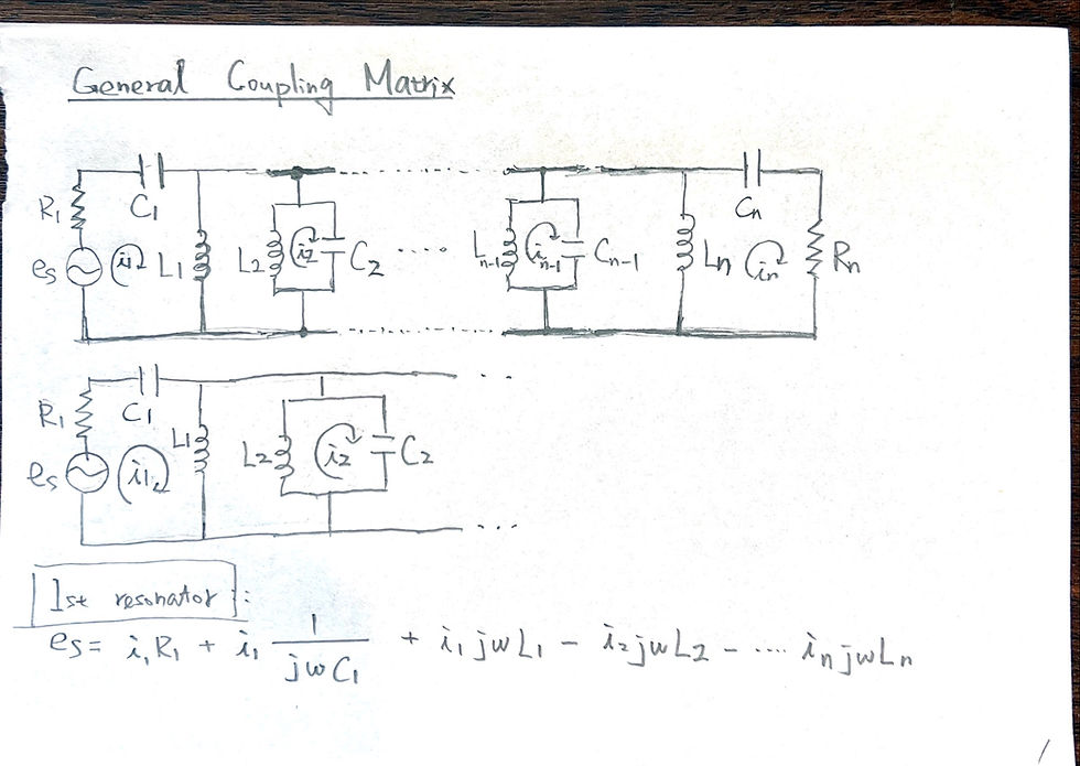
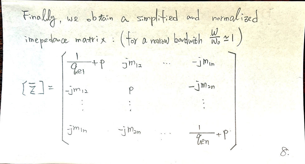
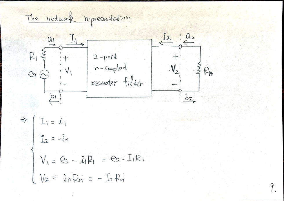
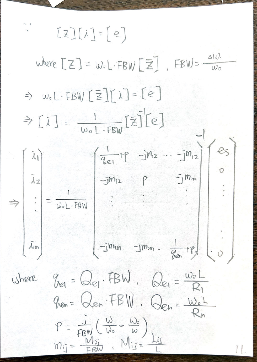
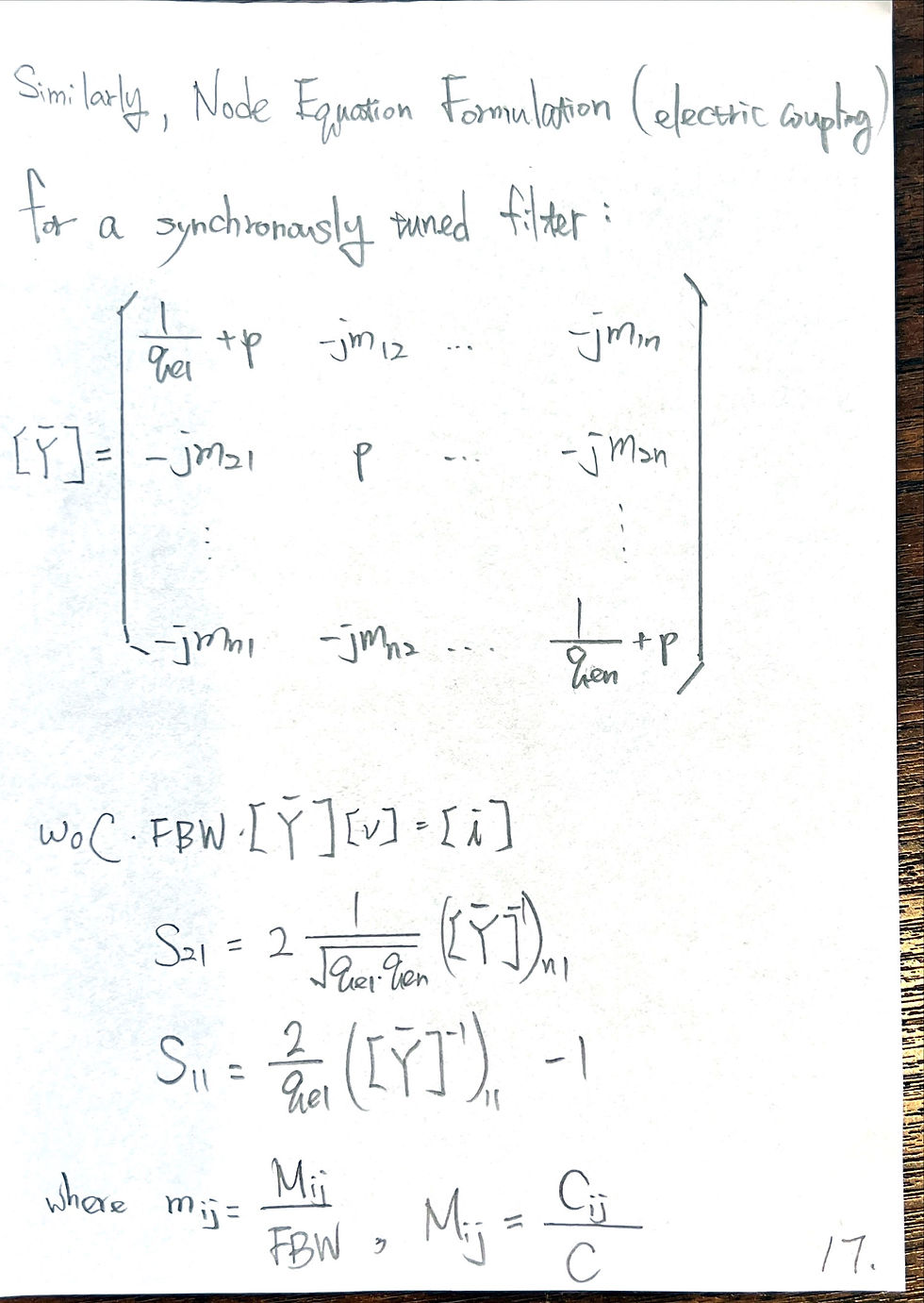
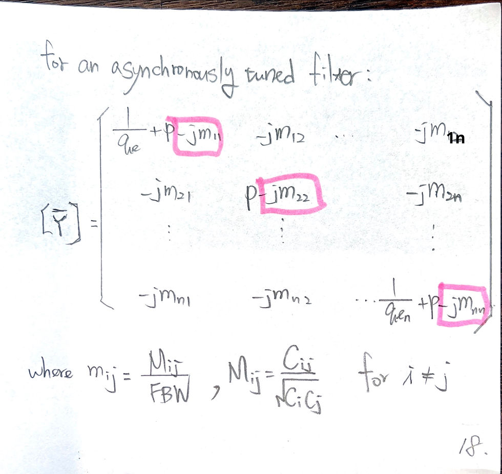
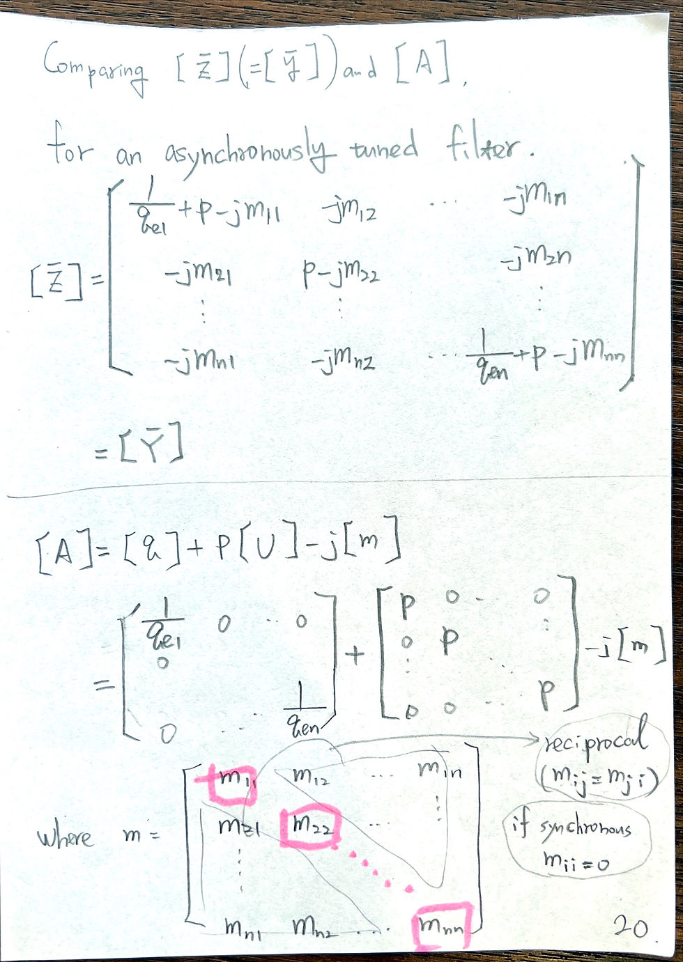
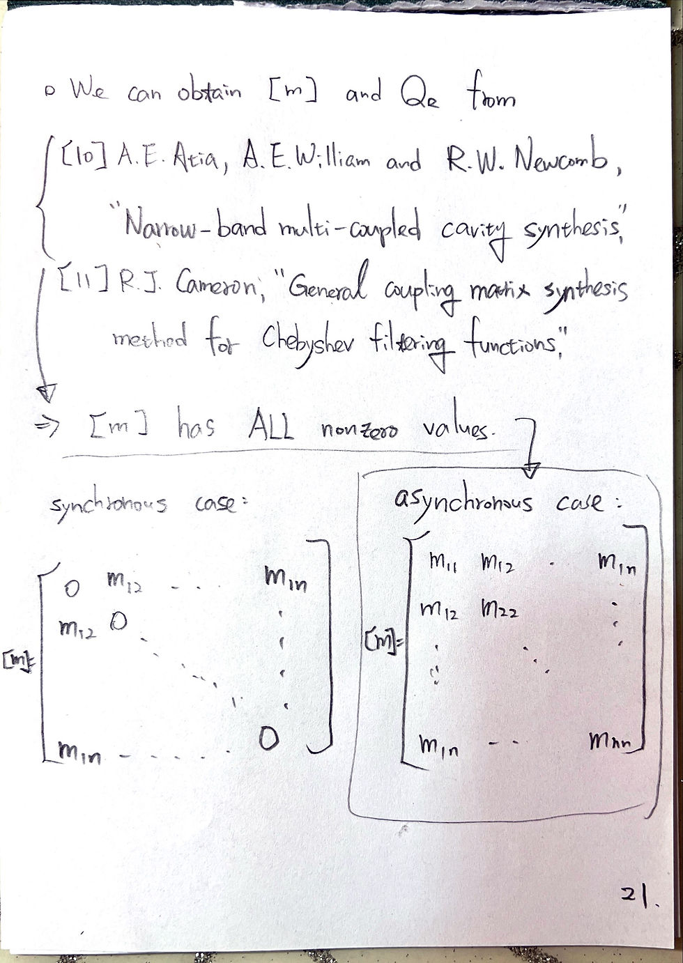
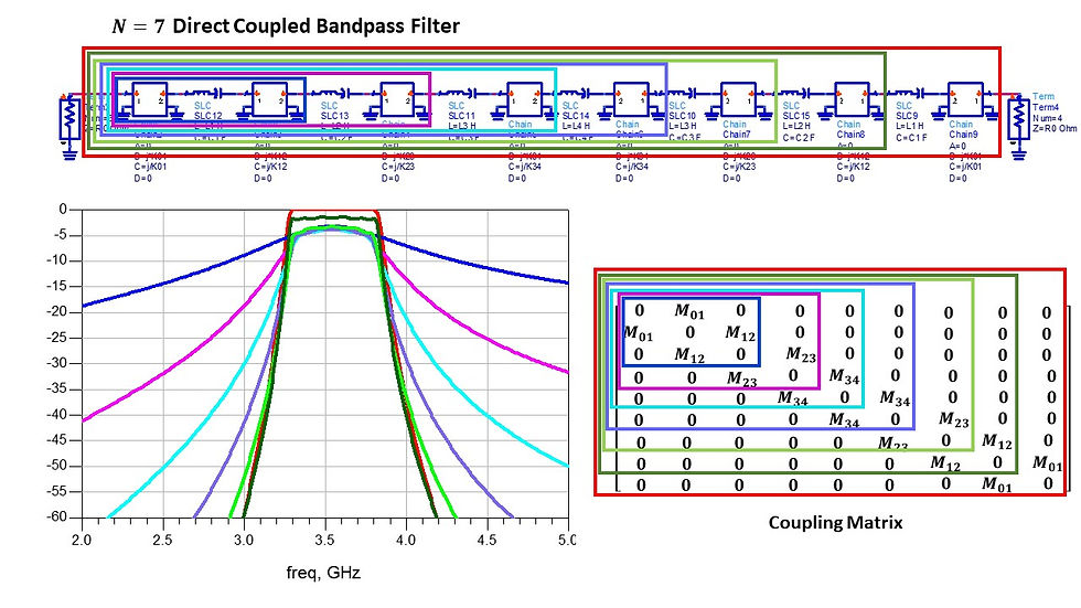
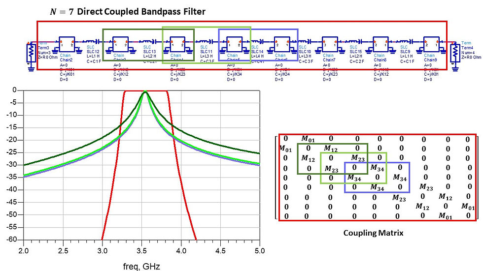
General Coupling Matrix

ㄨ

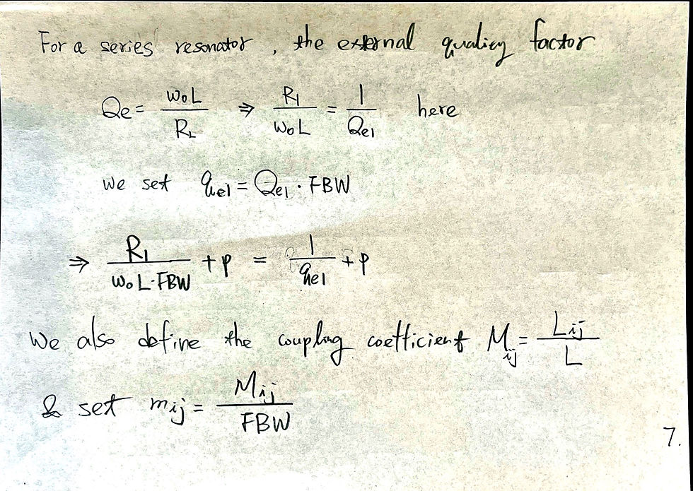
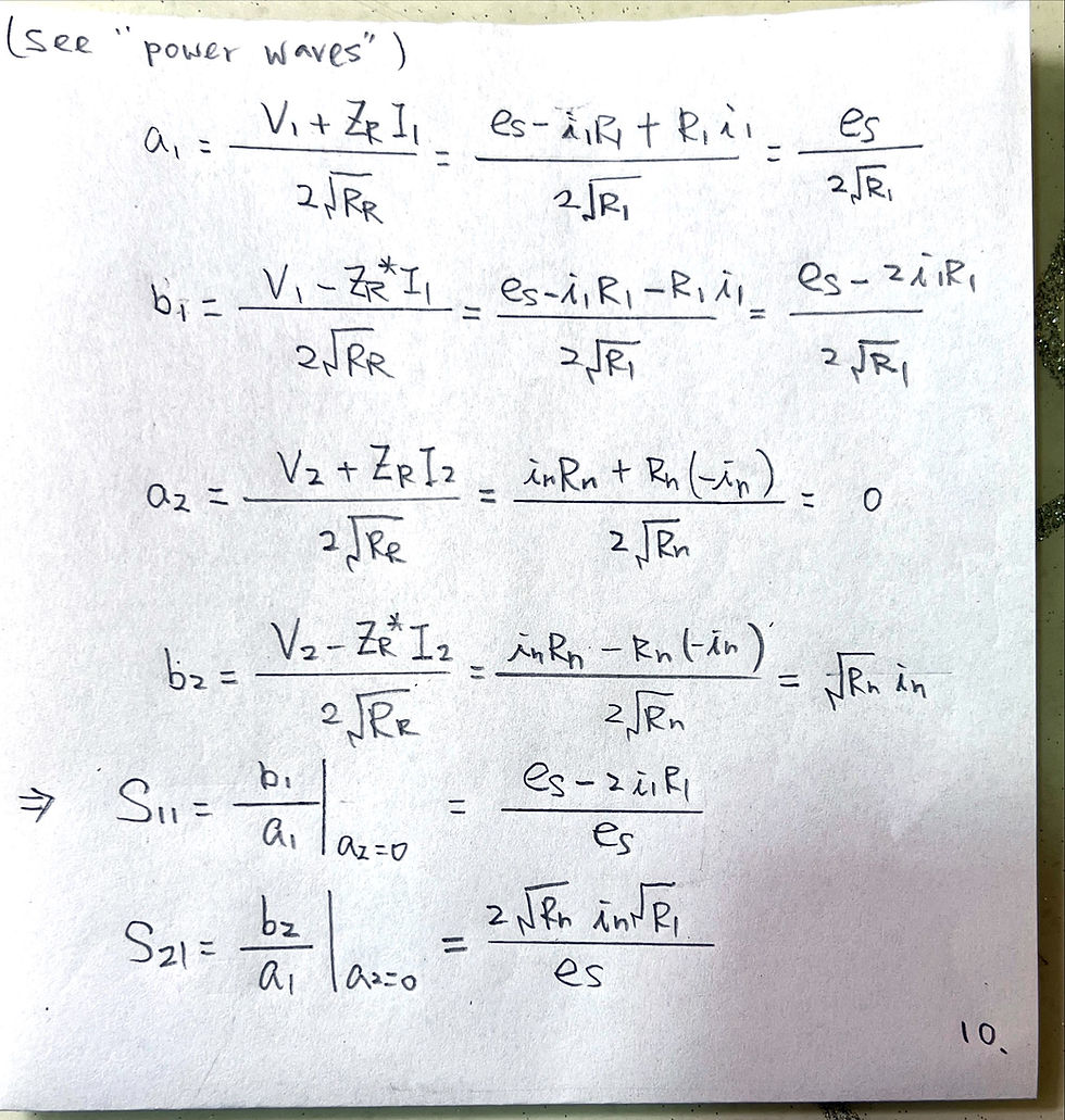
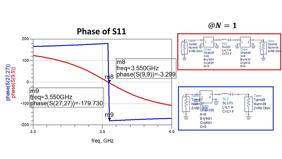
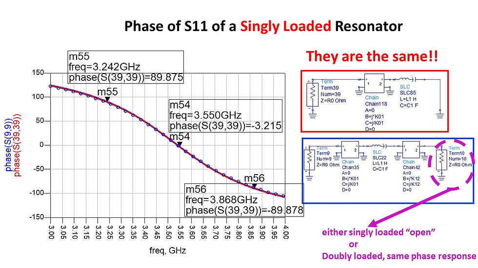
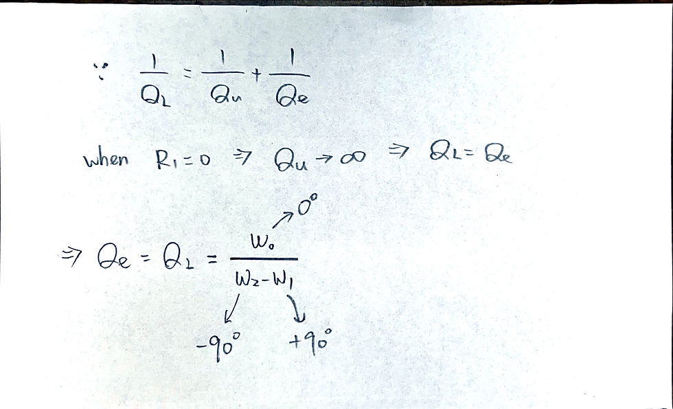
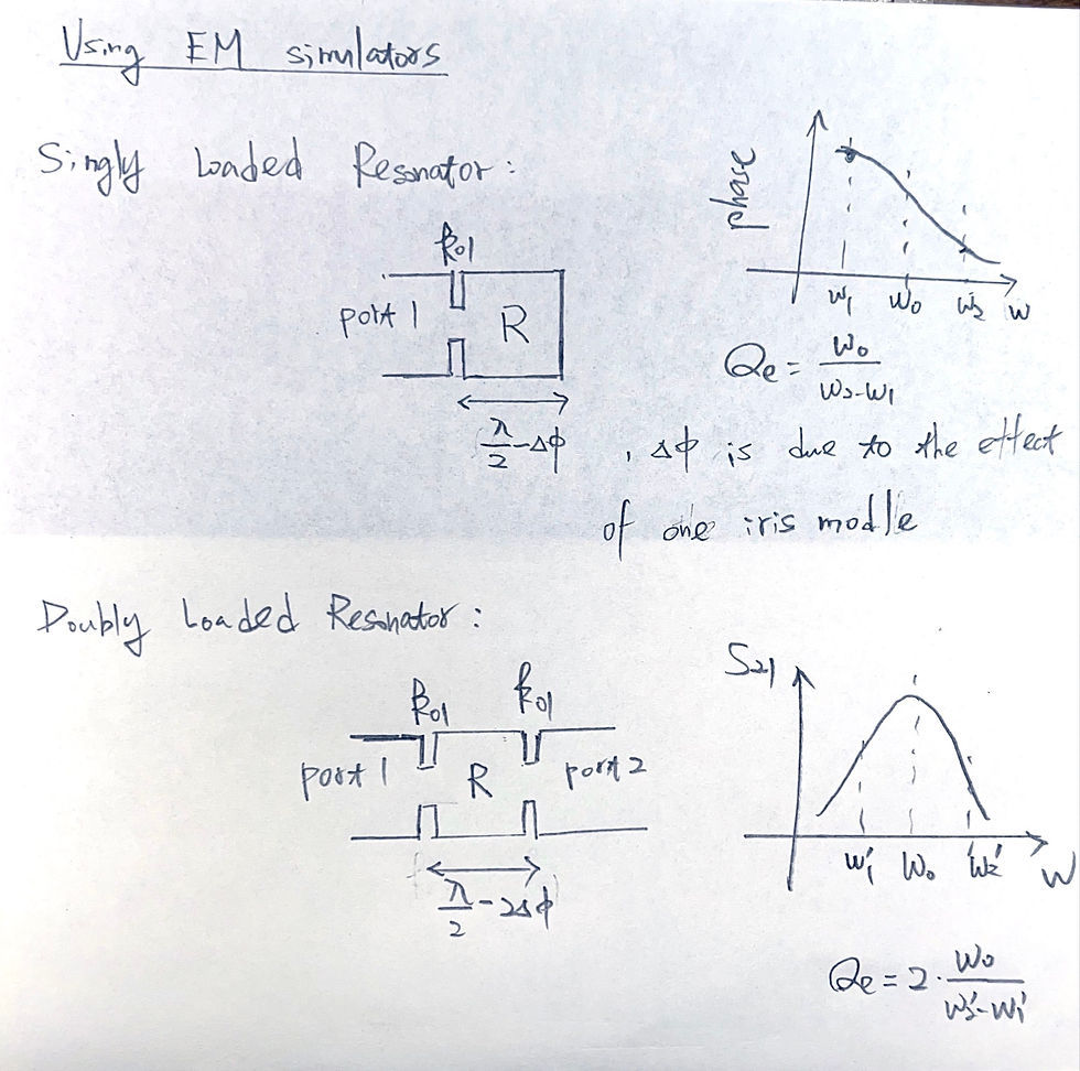
Conclusion of singly loaded resonator: use phase of S11 to fit Qe

In[2]:= 3.55/(3.868 - 3.242)

Out[2]= 5.67093

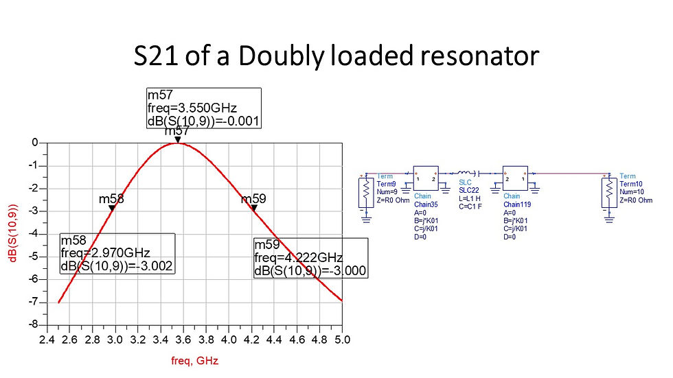
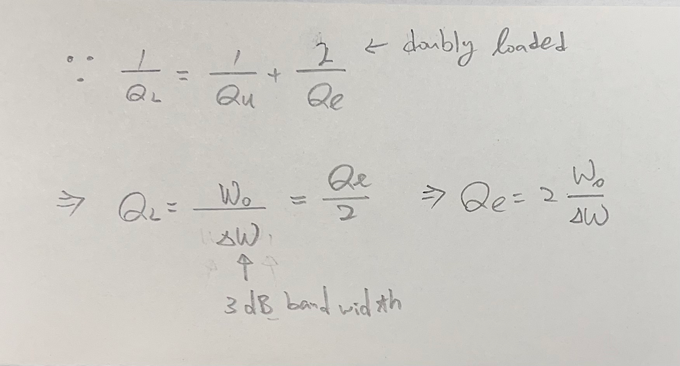
In[4]:= 2*3.55/(4.222 - 2.97)

Out[4]= 5.67093

a = 3.075*10^9;

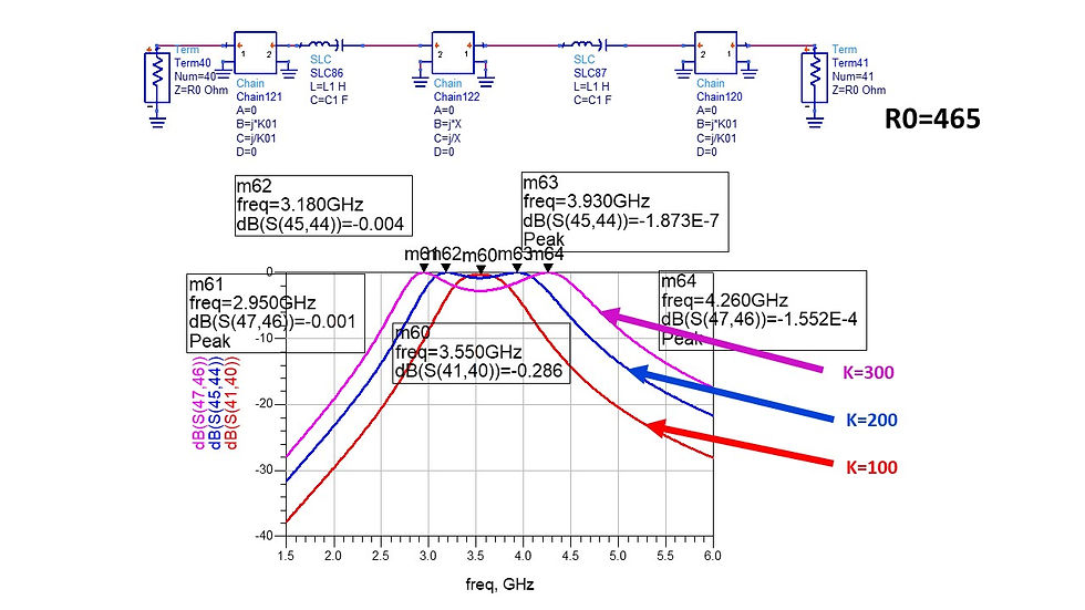
Z0 = 465;

w1 = 2*\[Pi]*3.3*10^9;

w2 = 2*\[Pi]*3.8*10^9;

w0 = Sqrt[w1*w2];

f0 = w0/(2*\[Pi]);

b = f0^2/a

L = Z0/w0*\[Pi]/2;

M = (b^2 - a^2)/(b^2 + a^2)

K = w0*L*M

4.07805*10^9

0.275045

200.899

w1 = 2*\[Pi]*3.3*10^9;

w2 = 2*\[Pi]*3.8*10^9;

w0 = Sqrt[w1*w2];

f0 = w0/(2*\[Pi]);

f[x_] := Z0*\[Pi]/2*((f0^2/x)^2 - x^2)/((f0^2/x)^2 + x^2);

g[x_] := Z0*\[Pi]/2*(x^2 - (f0^2/x)^2)/(x^2 + (f0^2/x)^2);

Plot[{f[x], g[x]}, {x, 0, 2.5*f0}, AxesLabel -> {"fp1&2", "K"},

AspectRatio -> 1, PlotStyle -> {Red, Blue}, PlotRange -> {0, 900}]

plot1 = ParametricPlot[{f[x], x}, {x, 0.001, f0}, AspectRatio -> 1,

PlotStyle -> Red];

plot2 = ParametricPlot[{g[x], x}, {x, f0, 2.5*f0}, AspectRatio -> 1,

PlotStyle -> Blue];

Show[plot1, plot2, AxesLabel -> {"K", "fp1&2"},

PlotRange -> {0, 8*10^9}]